Collider Bias in Applied Research

Ari Fenn, Researcher
March 31, 2021

When I was first taught regression analysis as an undergraduate, the first idea that was drilled into my head is that correlation is not causation. Essential to this discussion, the second idea was to control for possible bias. There are now many methods available to applied researchers to do causal research. For an approachable book on causal inference, see Cunningham (2021). These methods open additional biases that a researcher must consider and address, though this is not always a straightforward task.

Bias occurs in regression analysis when the estimated coefficient systematically differs from the population parameter being estimated. Most researchers are familiar with omitted variable bias (OVB), which occurs when a variable related to the outcome is left out of the regression. Some, or all, of the omitted variable’s effect is included in the coefficient of the variable of interest, making it a biased estimate of the population parameter. When establishing causal estimates, just as in correlational estimates, bias affects the magnitude and potentially the sign of the coefficient and does not allow for causal interpretations. Two types of biases are a confounder (OVB, etc.) and a collider.

I will use several highly stylized examples to demonstrate bias: one showing a confounder and two different types of colliders. These will abstract from variables other than those that are completely necessary to illustrate the basic ideas, assuming other characteristics only have a relationship with the outcome and are observable and can be controlled. I also assume the goal of the research project is causal interpretation.

Confounder

To demonstrate how bias affects estimates, I use directed acyclic graphs (DAG) (Pearl, 2009). The arrows show the direction of causation, and the pathways show where bias comes from.

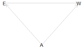
I start with an example of a confounder, Figure 1. Suppose we take education (E) and wages (W) where the arrow points from E to W, E → W shows that education raises wages by increasing diversity of skills and increasing productivity.

Imagine that ability (A) is a characteristic, such as intelligence, productivity, drive, or something similar. We might see that ability (A) influences both E and W, as in E←A→W. In this case:

• A can vary and move E and W.
• Due to A being without a control, this movement would bias any estimate of E with regards to W.

To control for A, we could use fixed effects or instrumental variables.

Collider as a control variable

Collider bias occurs when a variable the model is conditioned on is affected by both the outcome variable and one or more independent variables. If the arrows pointed to A, E→ A ← W, A is the collider. The only way that E becomes biased is if A is used in the model and opens the pathway that introduces bias.

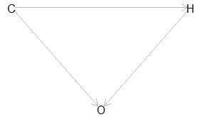
In Figure 2, we see the effect of unpaid household childcare hours (C) on work hours (H). Here the more unpaid care work that is done, the fewer or more irregular paid work hours are worked, C → H. But what if we also decide to include occupation (O)? In this case:

• Due to the care work (C), only certain occupations are available.
• Due to the irregular or part-time nature of the desired schedule (H), certain professions are not workable, so C → O ← H.

Now conditioning on an occupation opens a second path from care work to hours that would bias the effect of care work on hours.

Sample Selected on Collider

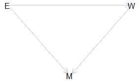
Collider bias can also enter more subtly for sample selection. In Figure 3, our wages and education information comes from an administrative data set with observations from one locality. The collider conditions which of the observations we see and these conditions can bias our estimated effect of education.

In this example, we have education (E) and wage (W) where education affects wage in the same manner as before, E → W. However, in this scenario, migration (M) out of the administrative area can occur. For example:

• More education makes one more attractive to potential employers outside the administrative area, so E → M.
• A higher wage makes it easier to exit the administrative area M ← W.

Migration (M) does not explicitly enter a regression equation to create the bias. However, it can still bias the effect of education on wages down as our model posited that the most educated and wealthiest are most likely to leave the area. This type of bias is much harder to adjust for.

How should one control for collider bias? Like all issues in applied research, collider bias may not be evident at first glance. It also may not always be a problem. Applied research should start with a theoretical model of how the world works. This model informs how the data is generated. By explicitly thinking through this process, one should ask if adding a variable opens pathways that create bias or if during the data collection, bias was introduced, as could be the case with administrative data.

For more complex examples of collider bias Gratz (2020) and Elwart and Winship (2014) discuss them in social sciences. To address bias in administrative data, I would read Know, Lowe, and Mummolo (2020). Hopefully, this discussion on bias will help make your research stronger.

All DAGs were made with dagitty for R.

References:

Elwert, F., & Winship, C. (2014). Endogenous selection bias: The problem of conditioning on a collider variable. Annual review of sociology, 40, 31-53.

Cunningham, S. (2021). Causal inference: The mixtape. Yale University Press.

Grätz, M. (2019). When Less Conditioning Provides Better Estimates: Overcontrol and Collider Bias in Research on Intergenerational Mobility (No. 2/2019). Stockholm University, Swedish Institute for Social Research.

Knox, D., Lowe, W., & Mummolo, J. (2020). Administrative records mask racially biased policing. American Political Science Review, 114(3), 619-637.

Pearl, J. (2009). Causality: Models, Reasoning, and Inference. Second Edition. Cambridge University Press.